by Amanda Rohrer
January 2013
Extreme weather events seem to be happening with increasing frequency and intensity. Hurricanes, 'snownami', and devastating tornadoes are all accompanied by an avalanche of media coverage. After the live weathercasts, scenes of devastation, and human interest stories, it's time for the coverage of economic implications. As the most recent such event, Hurricane Sandy, is credited with unusually high unemployment insurance claims, weak employment numbers, and poor holiday retail sales, it shines a spotlight on the fundamental problem of statistics: Although we can count the number of jobs, the number of workers employed and unemployed, and can even count the goods and services output, we have a lot more difficulty quantifying why and how. Why did employment in an industry grow for the year? Why did retail sales and hiring not keep up with expectations? How much impact does a disaster in our population centers have in surrounding regions, the nation, and the world?
To inform analysis, researchers and government agencies use a variety of methods to estimate the impact of economic events. Using multiple data sets is a common way of ensuring the significance of the occurrence; there should be noticeable effects in different measures for truly large-scale events. Comparing to similar known historical events, another tactic, helps to identify what we expect and to evaluate its scale. Another technique, and the focus of this article, is seasonal adjustment. While not specifically for analysis of major events, seasonal adjustment is invaluable for distinguishing the 'normal' from the 'abnormal' in economic trends.
Seasonal adjustment is a statistical method applied to time-series data that removes the usual fluctuations to leave only the trend. BLS FAQs defines it as follows:
Seasonal adjustment is a statistical technique which eliminates the influences of weather, holidays, the opening and closing of schools, and other recurring seasonal events from economic time series. This permits easier observation and analysis of cyclical, trend, and other nonseasonal movements in the data. By eliminating seasonal fluctuations, the series becomes smoother and it is easier to compare data from month to month.
For example, if school hiring usually increases employment in September, the seasonally adjusted series would discount that usual increase and show only how much more or less employment has grown. In a year where schools were cutting back and hiring fewer workers in September, the seasonally adjusted series would show a decline, despite the measured number of workers being higher over the month.
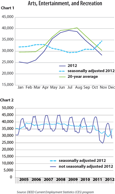
In Chart 1 seasonally adjusted data is plotted concurrently so the seasonal trend is apparent. While the level varies, the timing and magnitude of increases and decreases is largely consistent. The most recent seasonally adjusted series is included. During mid-2012 Arts, Entertainment, and Recreation employment grew rapidly. However, the industry always grows over the summer months, and because the growth was less substantial than usual, the seasonally adjusted series shows a decline in employment. In Chart 2 the time-series of seasonally adjusted and unadjusted data are shown together. While the seasonality of the unadjusted data is apparent, it swings so wildly over the course of the year that it makes it difficult to see the trend. The seasonally adjusted series, in contrast, removes those wild swings to show a trend that reflects recession-related and other economic events.
Seasonal adjustment doesn't assume all people work year-round. It doesn't even have much to do with weather - it's simply a method to separate the usual from the true economic trends so researchers and the public can better understand the economy of the present. Monthly employment numbers and unemployment rates are all released in both adjusted and unadjusted forms. The Consumer Price Index (CPI) and other common economic indicators are similarly published. Despite the widespread nature of the technique, it often sows confusion.
While Minnesota was not directly affected by Hurricane Sandy, we have experienced smaller scale weather events that have had an impact on our employment trends. Seasonal adjustment can help take our understanding of these adverse events beyond the anecdotal to the systematic.
For example, the 2011-12 winter was warm and nearly snowless. While salt-suppliers were pounded as roads needed little clearing, home improvement retailers and construction workers all started their seasons early. When they're celebrating St. Patrick's Day in t-shirts and by scooting around in golf carts, few people are worried about how much of the local economy depends on cold, snowy winters. Trucking firms, building maintenance, and city governments have to stockpile sand and salt in the fall to prepare for winter. If they guess quantities too low, and many did in 2010-11, they can run into late winter shortages and price spikes. In a warm and dry winter, when they buy too much, not only do they have the unrecoverable expense of excess sand and salt and potentially removal fees at the end of the winter if they have no long-term storage in the city, but workers whose winter paychecks are affected by weather are at risk. The truck drivers who deliver sand and salt, the plow drivers, and the snow-melt machine operators are all at risk of layoff. Their corollary summertime duties aren't yet needed, and employers are looking to make up the losses from overbuying materials.
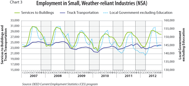
Because current employment numbers are available only by industry, we can't look at employment for just these occupations, but we can look at the industries in which most work. The most precise such industries are too small to be seasonally adjusted, but show an apparent weather effect. Services to Buildings declined somewhat less than usual in 2010-11 and more and for a longer time in 2011-12. Local government employment didn't see any of the second January peak that appears in all other years. Truck transportation dropped off comparatively little in 2010-11 but fairly rapidly in 2011-12. This includes all workers who received pay in the reference week, the week which includes the 12th of the month. It doesn't account for changes in hours or total pay, which may disguise some of the effect. For the industries that are large enough to be seasonally adjusted, the impact is further diminished.
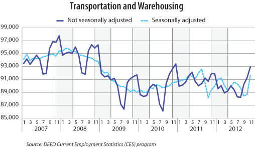
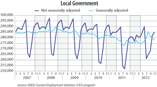
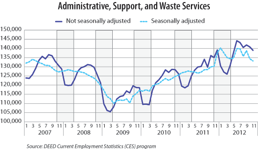
Chart 3 is a comparison of adjusted and unadjusted data for the three major industries that include sand and salt wholesalers and delivery, facilities maintenance workers, and city government workers who operate plows. Keep in mind that these are all large industries - only about 75 percent of Transportation and Warehousing employment is truck transportation and warehouses, and a large portion of that likely is shipping related to retail sales. Half of local government employment is in education and wouldn't be affected by trends in city services. Only 20 percent of Administrative, Support, and Waste services employment works in building maintenance. Even so, the seasonal adjustment of the larger industries can still be meaningful. In the winter of 2008-09 all of these industries declined on a seasonally adjusted basis, despite fairly normal weather conditions. Since that was during the recession when all industries were struggling, those declines were likely a result of the larger economic picture. However, in other average winters, seasonally adjusted employment figures were mostly level, indicating employment change that was as expected.
In winter 2010-11 Transportation and Warehousing saw steady increases in seasonally adjusted employment. Some is a product of ongoing economic growth, but the post-holiday drop-off in employment was less substantial than in other years. In 2011-12 employers hired many fewer workers in advance of the holidays, but laid them off at a normal rate, resulting in an over-the-year decrease. The seasonally adjusted series may be skewed by the timing of the benchmark revision and isn't easily explained. Local government employment in 2010-11 was weak, possibly because existing workers were offered overtime rather than new workers being hired. Budget gaps were made up in the following season, as local government employment declined more rapidly in the summer months than even during the recession, although this effect was compounded by ongoing budget troubles. Administrative, Support, and Waste Services was stronger than average throughout the 2010-11 winter, while 2011-12 appears to have stronger-than-normal hiring in anticipation of the winter but a rapid drop-off as workers lost their jobs at a faster-than-average seasonal rate. Analysis of seasonal adjustment may be more helpful after another annual benchmarking period. When they become available, more granular data sources like the Quarterly Census of Employment and Wages for changes both in employment and pay can be examined and would be another effective technique for understanding the economic effects of recent winters.
Abnormal weather isn't the only source of economic trends. Large events like the state government shutdown in July 2011 or the 2008 Republican National Convention may appear in the seasonally adjusted series as dips and increases of various sizes. Few events, however, are truly significant enough to appear. Often other irregular events balance them out with near comparable losses or gains. This is what makes seasonal adjustment such a useful tool - it reflects the overall trend without being substantially swayed by every minor variation.
The basic method, though, has some limitations. First, seasonal adjustment requires several years' worth of historical data to establish the trend, and the history should be as granular as the current series - where there are only annual averages or totals available historically, you cannot build a model of monthly seasonality. Second is the underlying series itself. Current monthly employment and unemployment rates, the measures that provide the most current state-level employment numbers, are estimates based on both survey data and outside inputs. To improve accuracy, outside inputs and projected values are updated and estimates are recalculated annually. As a result, the current (last one to three years) series is significantly more volatile than previous years, meaning the seasonal adjustment is similarly volatile (see charts for apparent volatility1). Third, to adapt to changing trends most seasonal adjustment processes give more weight to recent years. In abnormal times, this can skew the output. This is doubly troublesome because we often adjust modeled series since all include some kind of preliminary/predicted data that will be revised later. Those predicted inputs are based on past values as well, with a similar emphasis on recent years. This compounds the error in the prediction and makes re-estimation particularly critical. Fourth, seasonal adjustment is most meaningful when applied to large groups - large industries or geographic areas. Often, the most significant economic effects of an event are isolated to a much smaller corner of the economy.
The economy is a complex system with each occurrence rippling out to unpredictable end results. Although we have many analytical tools, understanding their implementation, their limitations, and their advantages is critical to understanding conclusions drawn from their use. Seasonal adjustment is one such tool. To interpret seasonally adjusted measures correctly, it's critical to have an understanding of the bigger picture.
1This topic is reviewed each re-estimation period. For an article on last year's benchmark changes, see the 2011 Benchmark Revisions and Their Effects on Two Programs article in the Minnesota Employment Review Archive.